Analysis Outputs: Descriptive & Exploratory
A guide to reading common descriptive plots and numerical summaries.


Descriptive and exploratory analysis summarises and describes the characteristics of a dataset, providing insight into distributions, central tendency, spread, and relationships between variables. It serves two closely related purposes: as a standalone way of characterising and communicating what the data shows, and as an essential first step before formal modelling or hypothesis testing. Used in this exploratory capacity, descriptive analysis helps reveal the shape and structure of your data, identify potential issues, and inform decisions about how best to proceed with formal analysis.
This guide covers the most common outputs from descriptive and exploratory analysis that you are likely to encounter, explaining what they represent, what different patterns indicate, and what types of data each is appropriate for. It is organised into two sections: plots and figures, which covers common visualisations used to explore and describe data, and numerical summaries, which covers the key statistics used to characterise and communicate the properties of a dataset.
Plots and Figures
Visualisations are one of the most powerful tools in data analysis, making patterns, distributions, and relationships visible in ways that raw numbers alone often cannot. Plots like histograms, boxplots, and scatter plots are particularly valuable during exploratory data analysis, helping to reveal the shape and spread of data, identify outliers, and assess relationships between variables. This guide covers the most common descriptive plot types you are likely to encounter, explaining what they represent, what different patterns indicate, and what types of data each is appropriate for.
Histograms
A histogram displays the distribution of a continuous variable by grouping values into intervals known as bins, and showing how many observations fall within each bin as a bar. The height of each bar represents the frequency of values in that range, making it easy to see at a glance where values cluster, how spread out they are, and whether any unusual patterns are present.
A key feature of a histogram is that the bars touch. This reflects the fact that the underlying data is continuous, meaning there are no gaps between possible values and therefore no gaps between bins. This distinguishes a histogram from a bar chart, which is used for discrete or categorical data where each bar represents a separate group rather than a range of a continuous scale. If your data consists of counts, ordinal scores, or named categories, a bar chart is the more appropriate choice.
Histograms are commonly used during exploratory data analysis to understand the distribution of a variable before any formal modelling takes place. They help reveal how spread out values are, whether they cluster around a central point, whether there are unusually high or low values, and whether the distribution is symmetrical or skewed. This kind of early understanding of your data is important for informing decisions about which analytical methods are likely to be appropriate.
Histograms are also widely used during and after model fitting to examine residuals, the differences between observed values and the values predicted by the model. Most common analytical methods require that residuals are approximately normally distributed, and plotting a histogram of residuals is a straightforward way to assess whether this holds. It is worth noting that it is the residuals rather than the raw data that need to follow an approximately normal distribution. Raw data can be skewed or non-normal and the residuals can still be approximately normal after a model is fitted. However, heavily non-normal raw data may be an early indication that this is worth checking carefully once a model has been fitted.
Reading histograms
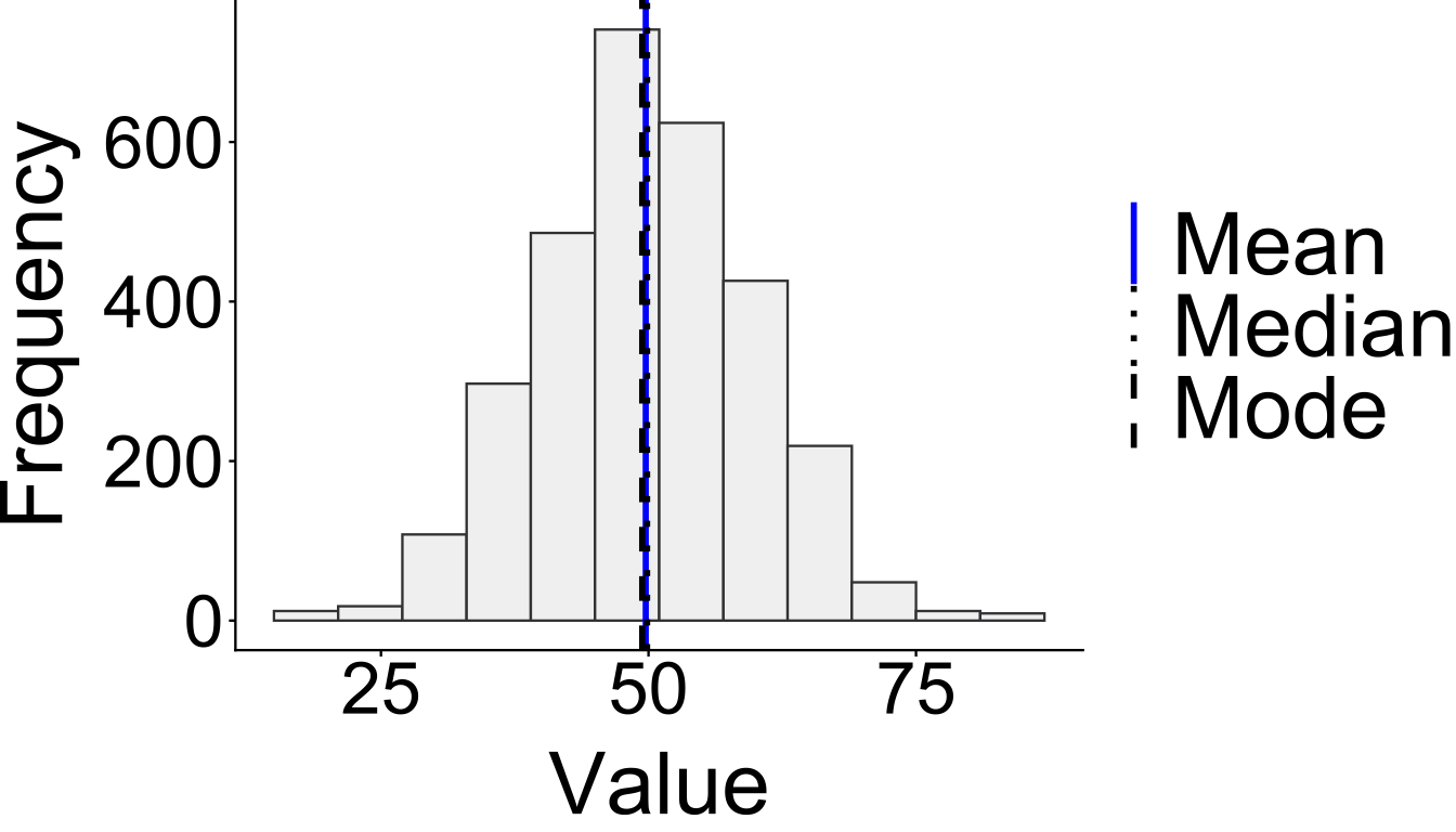
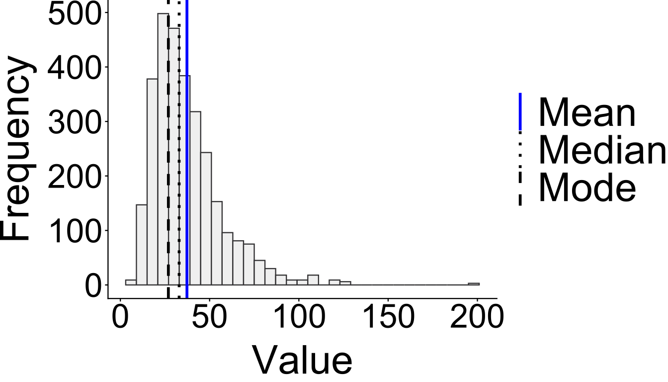
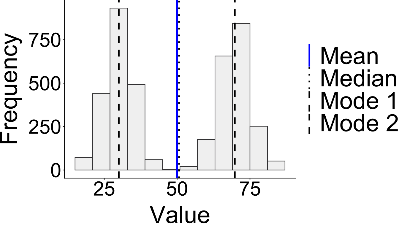
Look at where the bars are tallest, as this is where most values fall. A symmetrical bell-shaped curve suggests an approximately normal distribution, where values cluster evenly around a central point with the mean, median and mode all close together (Figure 1). A longer tail on one side indicates skewness. A right-skewed distribution has a tail extending to the right, meaning most values are lower with fewer very high values pulling the mean upward. A left-skewed distribution has a tail extending to the left, meaning most values are higher with fewer very low values pulling the mean downward (Figure 2). Two distinct peaks suggest the data may contain two subgroups with different underlying characteristics, known as a bimodal distribution, which is worth investigating further before proceeding with analysis (Figure 3). Bars sitting far from the main cluster may indicate outliers worth examining.
Boxplots
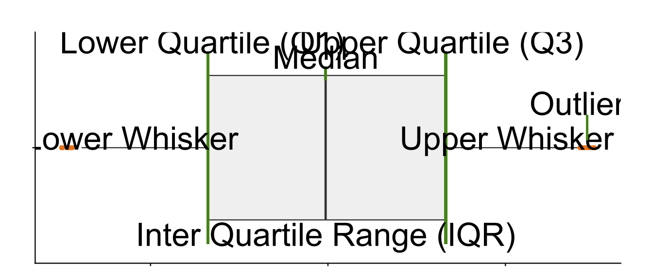
A boxplot, or box-and-whisker plot, summarises the distribution of a continuous variable by displaying key statistics including the median, quartiles, and potential outliers in a compact visual form. Boxplots are particularly useful in exploratory data analysis for understanding the spread and shape of your data, and for comparing distributions across groups.
Because the boxplot is built around the median and quartiles rather than the mean, it is not strongly influenced by extreme values. A single very high or very low observation can pull the mean substantially away from the centre of the data, but has little effect on the median or the box, making boxplots a reliable summary of your data’s distribution even when outliers are present.
It is worth noting that the 1.5 times IQR rule used to define the whiskers and flag potential outliers is a convention rather than a formal statistical test. Points plotted beyond the whiskers are not necessarily problematic but are worth examining in the context of your data. It is also worth being aware that boxplots do not convey sample size, meaning a box based on ten observations looks the same as one based on ten thousand.
Reading boxplots
When reading a boxplot, start with the median line. Its position within the box indicates whether the data is roughly symmetric or skewed. A median sitting centrally suggests an even distribution on both sides, while a median closer to one end of the box indicates that values are more concentrated on that side. The relative length of the whiskers tells a similar story; a longer whisker on one side suggests the data extends further in that direction.
A wide box indicates high variability in the middle 50% of values, while a narrow box suggests values are tightly clustered. The interactive examples above allow you to see how these features change across different distribution shapes, and how the same patterns identified in histograms appear differently when summarised as a boxplot.
Comparing groups
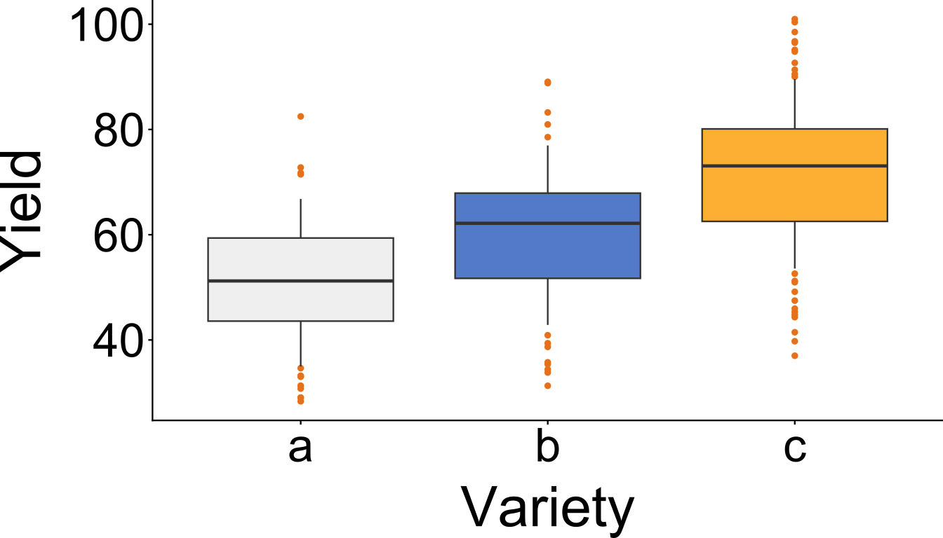
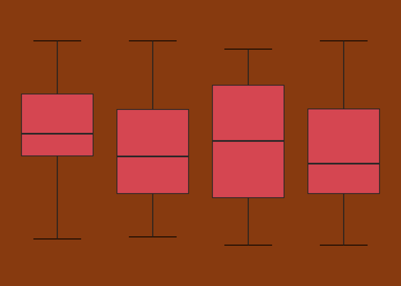
Where boxplots are most powerful is in side-by-side comparison (Figure 5). Differences in median position indicate differences in central tendency between groups. Differences in box width and whisker length indicate differences in spread. Overlapping boxes suggest groups may not differ meaningfully, while clearly separated boxes suggest real differences worth investigating further.
Scatter Plots
A scatter plot displays the relationship between two numeric variables by plotting individual observations as points, with one variable on each axis. It is most appropriate when both variables are measured on a continuous scale, making it easy to see at a glance whether a relationship exists, what direction it takes, and how strong it appears to be.
Scatter plots are particularly valuable during exploratory data analysis as an early step before formal modelling. Seeing the shape of the relationship between two variables helps inform which analytical methods are likely to be appropriate.
Reading scatter plots
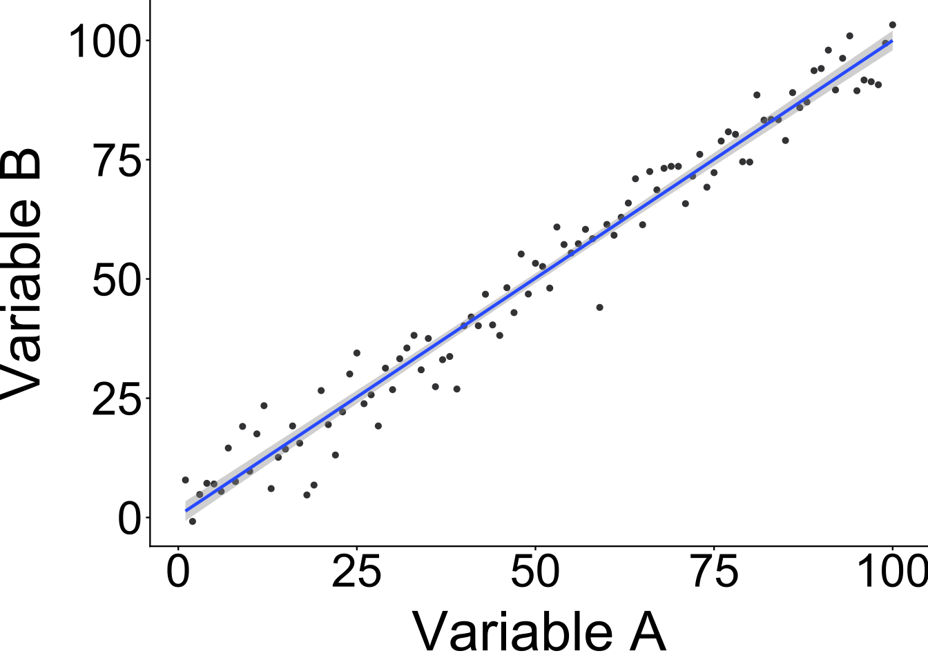
Start with the overall pattern. Points forming an upward trend indicate a positive relationship, where higher values of one variable tend to coincide with higher values of the other. A downward trend indicates a negative relationship. A random scatter with no clear direction suggests little or no relationship between the variables.
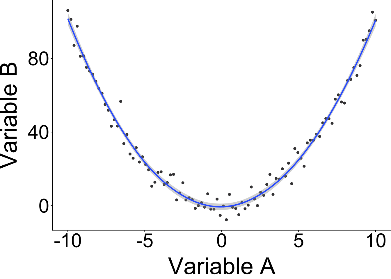
The closeness of points to an imaginary or fitted line reflects the strength of the relationship. Points clustering tightly around a clear trend indicate a strong relationship, while a more dispersed pattern suggests a weaker one. It is also worth looking at whether the relationship is linear, following a straight line, or non-linear, following a curve, as this affects which analytical methods are appropriate (Figure 6, Figure 7).
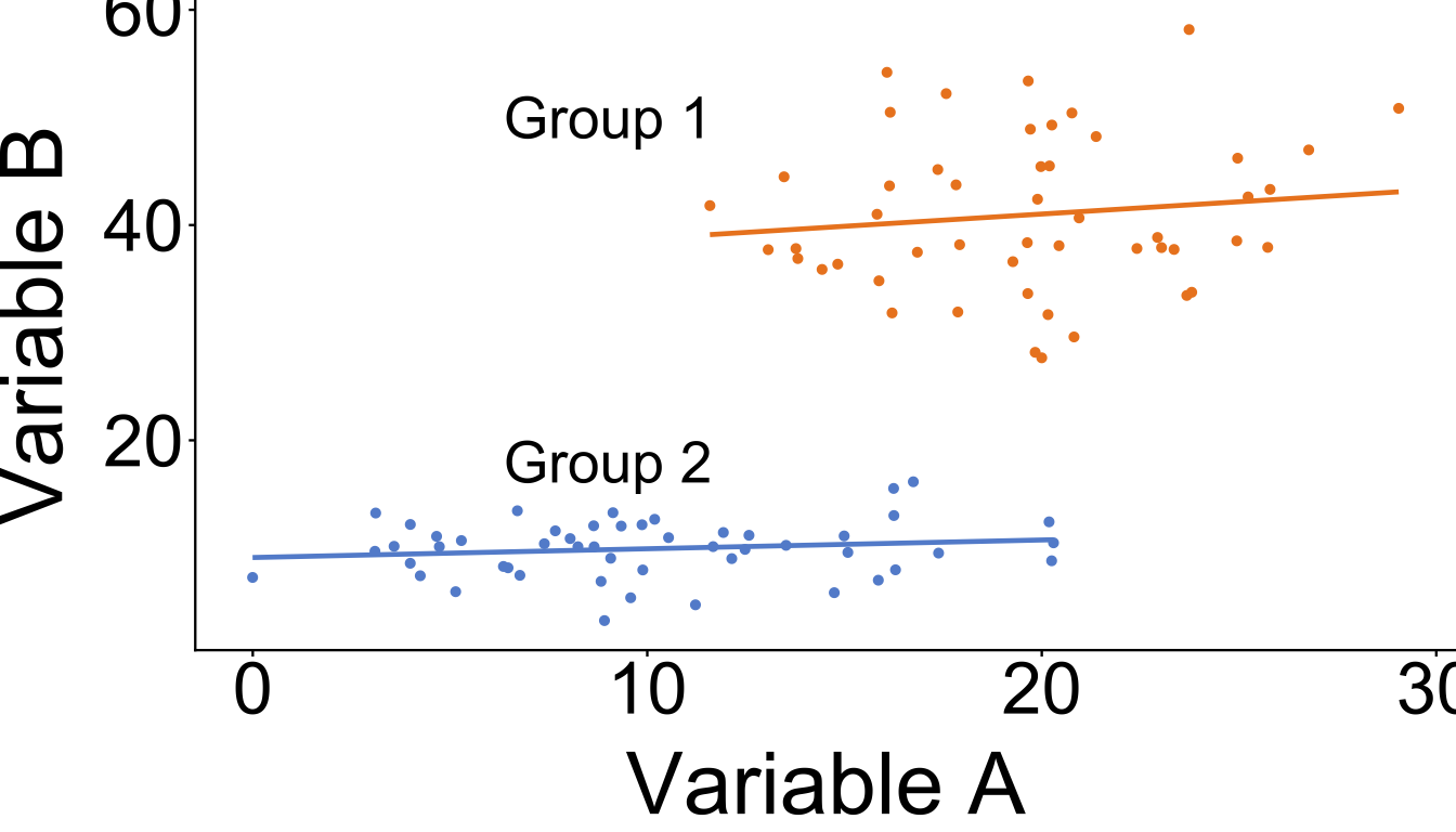
Where points fall into distinct clusters or groups, analysing them as a single trend can be misleading. If a grouping variable is present in your data, it is worth plotting groups separately or using colour to distinguish them, as different groups may show quite different relationships (Figure 8).
With large datasets, points can overlap heavily, making it difficult to see the true density and distribution of observations. If a scatter plot looks unusually sparse or clustered in a way that seems inconsistent with the data, overplotting may be obscuring the true pattern.
Points sitting far from the main cluster may be outliers worth investigating. It is also important to remember that a relationship visible in a scatter plot indicates association, not causation. Two variables can be strongly correlated without one causing the other, and apparent relationships can sometimes reflect the influence of a third variable not included in the plot.
Numerical Summaries
Numerical summaries complement visualisations by providing precise, comparable values for the key properties of a dataset. Where a plot gives an overall impression of shape and spread, a numerical summary gives exact values for central tendency, variability, and composition. The two are most useful together: a plot reveals patterns and structure that numbers alone can obscure, while numerical summaries provide the precision needed for interpretation and reporting.
Means
The mean is the most commonly used measure of central tendency. It is calculated by summing all values in a variable and dividing by the number of observations, producing a single number that represents the typical or average value in the dataset. The mean is appropriate for continuous numeric variables — it is not meaningful for categorical data, where values represent groups or labels rather than quantities.
The mean is sensitive to extreme values. A single very high or very low observation can pull the mean substantially away from the centre of the data, giving the impression that the typical value is higher or lower than it actually is for most observations. In a right-skewed distribution, the mean is pulled upward by the long tail, sitting above the median and above the bulk of the data. In a left-skewed distribution, it is pulled downward in the same way.
When a distribution is approximately symmetric and free of extreme values, the mean is a reliable and informative summary of the centre. When the data is skewed or contains outliers, the median is often more appropriate, as it is not affected by extreme values in the same way. Comparing the mean and median directly is itself informative: when they are close together, the distribution is roughly symmetric; when they diverge, skewness or the influence of outliers is likely.
Standard Deviations
The standard deviation measures how spread out values are around the mean. A small standard deviation indicates that values cluster tightly around the mean, while a large standard deviation indicates that values are more widely dispersed. It is expressed in the same units as the original variable, making it directly interpretable alongside the mean. Like the mean, it is appropriate for continuous numeric variables and is not meaningful for categorical data.
Like the mean, the standard deviation is sensitive to extreme values. A single outlier can inflate it substantially, making the data appear more variable than it is for most observations. For skewed or heavy-tailed distributions, the interquartile range — visible in a boxplot as the width of the central box — is often a more robust and informative measure of spread, as it describes variability in the middle 50% of values without being affected by the extremes.
Where the distribution is approximately normal, the standard deviation has a well-established interpretive relationship with the data. Approximately 68% of values will fall within one standard deviation of the mean, approximately 95% within two, and approximately 99.7% within three. This makes it particularly useful for communicating what a typical range of values looks like, and for identifying observations that fall unusually far from the centre.
Frequency Tables
A frequency table summarises how often each value or category appears in a dataset, listing each unique value or group alongside a count of the observations it contains. Frequency tables are most commonly used for categorical or discrete variables, where the number of distinct values is small enough to list meaningfully.
They often include relative frequencies alongside raw counts, expressing each count as a proportion or percentage of the total. Relative frequencies are more informative than raw counts when comparing groups of different sizes, as they allow fair comparison regardless of how many observations each group contains.
Reading a frequency table involves looking for the values or categories that appear most often, assessing whether values are spread relatively evenly or concentrated in a small number of categories, and noting any counts that seem unexpectedly high or low. A category with a surprisingly high or low count compared to what would be expected is worth investigating, as it may reflect genuine patterns in the data or indicate issues with coding or data collection.
Frequency tables are particularly useful during the early stages of data checking, before any formal analysis begins. Examining the distribution of each variable this way can surface unexpected values, miscoded entries, or implausible counts that are worth resolving before proceeding.